Optimization of Distributed Joins
Challenges of Joins
For the 3-table join $R(A, B) \bowtie S(B, C) \bowtie T(C)$, there is a decision to make about which two of them to join first.
| R(A, B) | |
|---|---|
| 1 | 1 |
| 2 | 1 |
| 3 | 2 |
| 4 | 2 |
| S(B, C) | |
|---|---|
| 1 | 1 |
| 1 | 2 |
| 1 | 3 |
| 1 | 4 |
| T(C) |
|---|
| 3 |
| 5 |
$R(A, B) \bowtie S(B, C)$ creates a big intermediate result of 8 tuples below, where only 2 highlighted in red eventually survive in the final join result. The steep network cost of transmitting the redundancy makes it even more undesirable in a distributed setting.
| R(A, B) ⋈ S(B, C) | ||
|---|---|---|
| 1 | 1 | 1 |
| 1 | 1 | 2 |
| 1 | 1 | 3 |
| 1 | 1 | 4 |
| 2 | 1 | 1 |
| 2 | 1 | 2 |
| 2 | 1 | 3 |
| 2 | 1 | 4 |
| S(B, C) ⋈ T(C) | ||
|---|---|---|
| 1 | 3 | |
An alternative choice to process $S(B, C) \bowtie T(C)$ first is better, as it leaves only 1 tuple that contributes to the final join result.
Assuming each table is stored on a different node, we still need to ship many redundant tuples to execute $S(B, C) \bowtie T(C)$. Is there a way to cut down the network cost?
Exact Semi-joins
A semi-join $R \ltimes S$ keeps only the tuples in $R$ that also appear in $S$. Say we have two single-column tables $R(A)$ and $S(A)$.
| R(A) |
|---|
| 1 |
| 2 |
| 3 |
| 4 |
| S(A) |
|---|
| 2 |
| 4 |
The semi-join $R \ltimes S$ keeps only $\color{red}{2, 4}$ in R who also appear in S.
Yannakakis Algorithm uses semi-joins to filter out every irrelevant tuple, so that the join is executed later on the pruned tables with many fewer tuples.
Take the 3-table join $R(A, B) \bowtie S(B, C) \bowtie T(C)$ as an example again.
| R(A, B) | |
|---|---|
| 1 | 1 |
| 2 | 1 |
| 3 | 2 |
| 4 | 2 |
| S(B, C) | |
|---|---|
| 1 | 1 |
| 1 | 2 |
| 1 | 3 |
| 1 | 4 |
| T(C) |
|---|
| 3 |
| 5 |
The semi-join $S \ltimes T$ finds it enough to only consider the tuple $(1, 3)$ in $S(B, C)$. Another semi-join $R \ltimes S$ finds $(1, 1)$ and $(2, 1)$ in $R(A, B)$. $T \ltimes S$ finds $(3)$ in $T(C)$. After pruning, we only need to consider the highlighted tuples while executing the 3-table join.
Now the questions are
- How to run semi-joins faster & more compactly?
- In what order to perform those semi-joins?
Compact Bloom Filter for Fast Membership Queries
A semi-join is a batch of membership queries.
Bloom filter is a space-efficient probabilistic data structure for fast membership queries.
Two key components of a Bloom filter are a bit array and some hash functions. Say we start with a bit array of size $10$ and $2$ hash functions,
\[h_1(x) = x \bmod 10;\quad h_2(x) = (x + 4) \bmod 10.\]Initially, all the bits are set to $0$, meaning no element has been inserted yet.
| Index | 0 | 1 | 2 | 3 | 4 | 5 | 6 | 7 | 8 | 9 |
|---|---|---|---|---|---|---|---|---|---|---|
| Bit | 0 | 0 | 0 | 0 | 0 | 0 | 0 | 0 | 0 | 0 |
To insert 1,
because $h_1(1) = 1$ and $h_2(1) = 5$,
the bits at positions 1 and 5 are set to $1$.
| Index | 0 | 1 | 2 | 3 | 4 | 5 | 6 | 7 | 8 | 9 |
|---|---|---|---|---|---|---|---|---|---|---|
| Bit | 0 | 1 | 0 | 0 | 0 | 1 | 0 | 0 | 0 | 0 |
To insert 3,
because $h_1(3) = 3$ and $h_2(3) = 7$,
the bits at positions 3 and 7 are set to $1$.
| Index | 0 | 1 | 2 | 3 | 4 | 5 | 6 | 7 | 8 | 9 |
|---|---|---|---|---|---|---|---|---|---|---|
| Bit | 0 | 1 | 0 | 1 | 0 | 1 | 0 | 1 | 0 | 0 |
The query of 3 returns true positive,
as the bits at positions 3 and 7 are both $1$.
The query of 5 returns true negative,
as the bit at position $h_1(5) = 5$ is $1$ but that at $h_2(5) = 9$ is $0$.
The query of 7 returns false positive.
Though it is never inserted,
the bits at positions $h_1(7) = 7$ and $h_2(7) = 1$ both have been set
to $1$ by the insertions of some other elements.
The time & space efficiency of Bloom filter comes at the cost of accuracy. Hash collisions result in false positives.
Increasing the filter size reduces the false positive rate.
In an array of $m$ bits, a hash function supposedly maps uniformly to one of the $m$ bits. So it sets a bit to $1$ with a probability of $P_{1} = \frac{1}{m}$ and leaves a bit unchanged with $P_{0} = 1 - \frac{1}{m}$.
Assuming $k$ independent hash functions of a Bloom filter, the probability that a bit remains $0$ after inserting an element is
\[P_{0}^k = (1 - \frac{1}{m})^k.\]After inserting all $n$ elements, the probability that a bit remains $0$ is
\[P_{0}^{k \cdot n} = (1 - \frac{1}{m})^{k \cdot n}.\]Then the probability of a bit being set to $1$ is
\[P_{set} = 1 - P_{0}^{k \cdot n} = 1 - (1 - \frac{1}{m})^{k \cdot n}.\]The query of an element that’s never been inserted returns false positives if all of the $k$ bits it’s hashed to have been set to $1$. It gives us the false-positive rate, a.k.a. the error rate,
\[P_e = P_{set}^k = [1 - (1 - \frac{1}{m})^{k\cdot n}]^{k}.\]With the exponential approximation $\lim_{m \to \infty}(1 - \frac{1}{m})^m = e^{-m}$, we have
\[P_e \approx [1 - e^\frac{-k\cdot n}{m}]^{k}.\]Given $n$ inserted elements and $k$ hash functions, increasing the filter size $m$ reduces the false positive rate $P_e$.
Optimal Setup
A Bloom filter is a bit array where each bit is binary, either 0 or 1. It contains the maximum information per bit, measured by entropy, when half-full, i.e. $P_{set} = \frac{1}{2}$.
\[1 - (1 - \frac{1}{m})^{k \cdot n} = \frac{1}{2}\] \[\Downarrow\] \[{k \cdot n} \cdot \log(1 - \frac{1}{m}) = -\log(2)\]Because $\lim_{m\to \infty}\log(1 - \frac{1}{m}) = - \frac{1}{m}$,
\[\Downarrow\] \[m \approx \frac{k\cdot n}{\log(2)}.\]Distributed Approximate Semi-joins
The very purpose of semi-joins is to prune the tables.
If we don’t need to filter out every irrelevant tuple, Mackert and Lohman finds the compact Bloom filters an answer to fast membership queries. Bloom filters are easy to compute locally on each node. Thanks to their compactness, they are cheap to transmit over the network in a distributed database.
It only gives false positives for membership queries, so it doesn’t prune too hard to exclude any legit tuple from the final join result.
For the 3-table join above, if we were using a Bloom filter built on $T(C)$ to do an approximate semi-join $\tilde{\ltimes}$ that filters out some irrelevant tuples from $S(B, C)$ but leaving some false-positives, say $\color{orange}(1, 4)$, the final join would remain correct.
| R(A, B) | |
|---|---|
| 1 | 1 |
| 2 | 1 |
| 3 | 2 |
| 4 | 2 |
| S(B, C) | |
|---|---|
| 1 | 1 |
| 1 | 2 |
| 1 | 3 |
| 1 | 4 |
| T(C) |
|---|
| 3 |
| 5 |
Avoid Unnecessary Semi-joins
Mullin notices that some (approximate) semi-joins are totally unnecessary, like in our 3-table join $S \tilde{\ltimes} R$ that does NOT filter out a single tuple from $S$.
His solution is to partition one big Bloom filter into multiple smaller ones, send them one-by-one over the network and terminate this approximate semi-join between two nodes (supposedly hosting two tables) once a small partitioned filter fails to filter out enough irrelevant tuples.
How many is enough? A rule of thumb is that the size of irrelevant tuples needs to outweigh that of the partitioned filter to justify the communication cost.
How to partition? $k$ filters each of size $\frac{m}{k}$.
The error rate mentioned above for a Bloom filter of size $m$ with $k$ hash functions and $n$ elements inserted is
\[P_e = [1 - (1 - \frac{1}{m})^{k\cdot n}]^{k}.\]If we were using $k$ partitioned Bloom filters of smaller size $m’$ each with only 1 hash function, the error rate would be
\[P'_e = [1 - (1 - \frac{1}{m'})^{n}]^{k}.\]To achieve the same error rate, let $P_{set} = P’_{set}$,
\[[1 - (1 - \frac{1}{m})^{k\cdot n}]^{k} = [1 - (1 - \frac{1}{m'})^{n}]^{k}\] \[\Downarrow\] \[(1 - \frac{1}{m'}) = (1 - \frac{1}{m})^{k}\]By Taylor Expansion,
\[\Downarrow\] \[(1 - \frac{1}{m'}) = (1 - \frac{1}{m})^{k} = 1 - \frac{k}{m} + \frac{k(k-1)}{2m^2} + \cdots\]The filter size is usually much larger than the number of hash functions $m \gg k$,
\[\Downarrow\] \[(1 - \frac{1}{m'}) \approx 1 - \frac{k}{m} + O(\frac{1}{m^2})\] \[\Downarrow\] \[m' \approx \frac{m}{k}.\]Refining Approximate Semi-joins
Network is costly, while local computation is cheap. Upon receiving a Bloom filter from the previous node, the current node can refine that filter locally with a cheap bitwise AND operations and pass on the refined filter to the next node.
Say we are joining three single-column tables, the first one with two tuples $1, 2$ and the second one with $2, 3$.
The two hash functions, $h_1(x) = x \bmod 10$ and $h_2(x) = (x + 4) \bmod 10$, would give us the Bloom filters below:
| BF1 | 0 | 1 | 2 | 3 | 4 | 5 | 6 | 7 | 8 | 9 |
|---|---|---|---|---|---|---|---|---|---|---|
| Bit | 0 | 1 | 1 | 0 | 0 | 1 | 1 | 0 | 0 | 0 |
| BF2 | 0 | 1 | 2 | 3 | 4 | 5 | 6 | 7 | 8 | 9 |
|---|---|---|---|---|---|---|---|---|---|---|
| Bit | 0 | 0 | 1 | 1 | 0 | 0 | 1 | 1 | 0 | 0 |
Local bitwise AND gives us the refined filter:
| BF1&2 | 0 | 1 | 2 | 3 | 4 | 5 | 6 | 7 | 8 | 9 |
|---|---|---|---|---|---|---|---|---|---|---|
| Bit | 0 | 0 | 1 | 0 | 0 | 0 | 1 | 0 | 0 | 0 |
It contains the information of the tuples appearing in both tables and can be passed on to the third table.
Ramesh sees two ways to refine the approximate semi-joins in a master-slaves (or user-sites) distributed database such as the one below, where
- $Site_k$ stores table $T_k$;
- $BF_{i,j,k}$ is a Bloom filter refined by $T_i$, $T_j$, $T_k$;
- $RS_{i,j,k}$ is the (pruned) join result of $T_i$, $T_j$, $T_k$.
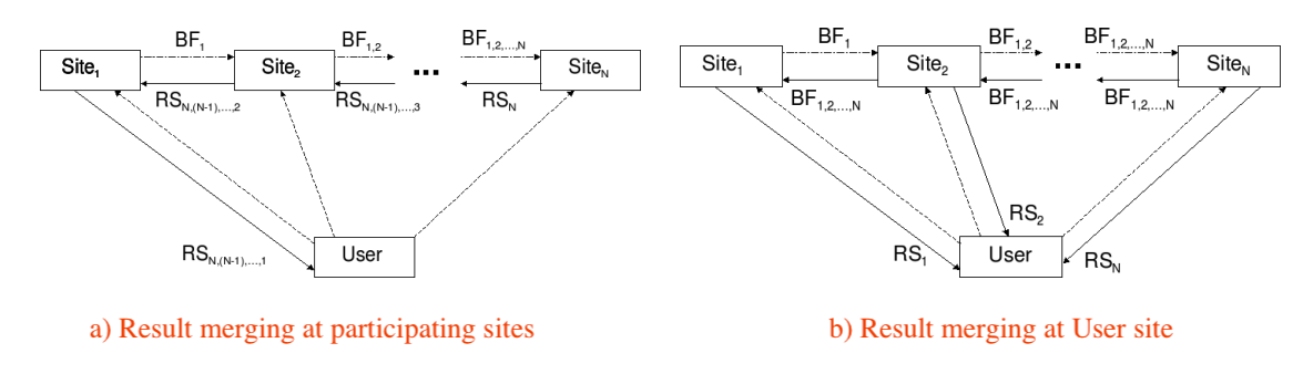
The scheme (a) refines the Bloom filters in one pass from $Site_1$, $Site_2$ to $Site_N$ in a cascading manner. It then incrementally computes the join result in a reversed pass from $Site_N$ back to $Site_1$ before returning the final join result to the user.
The scheme (b) refines the Bloom filters in two passes, first left-to-right from $Site_1$, $Site_2$ to $Site_N$ and then right-to-left. Each site then uses the highly refined filter at hand to return a pruned table to the user who eventually computes the final join result.
The network cost is the main concern when we determine the order of those approximate semi-joins. The scheme (a) uses that order for semi-joins and the (reversed) same order for computing joins incrementally. The scheme (b) has the flexibility of adopting a totally different order when the user executes the final joins.
Predicate Transfer for Distributed Joins
Joins are not always on the same attribute, like the running example of 3-table join $R(A, B) \bowtie S(B, C) \bowtie T(C)$, where the local bitwise-AND operations are not enough.
Predicate Transfer extends the Bloom-filter-powered approximate semi-joins to different attributes across multiple tables.
For example, when we consider a left-to-right pass $S := S \tilde{\ltimes} R$,
$T := T \tilde{\ltimes} S$ (and assume no false positive).
A Bloom filter on $R(B)$ is shipped behind the scene
to $S(B, C)$ to filter out $(3, 4)$ and
another Bloom filter on the pruned $S(C)$ to
$T(C)$ to filter out $(5)$.
| R(A, B) | |
|---|---|
| 1 | 1 |
| 2 | 1 |
| 3 | 2 |
| 4 | 5 |
| S(B, C) | |
|---|---|
| 1 | 3 |
| 1 | 2 |
| 2 | 3 |
| 3 | 4 |
| T(C) |
|---|
| 3 |
| 5 |
Another right-to-left pass $S := S \tilde{\ltimes} T$ and
$R := R \tilde{\ltimes} S$ further filters out $(1, 2)$ from $S(B, C)$
and $(4, 5)$ from $R(A, B)$.
| R(A, B) | |
|---|---|
| 1 | 1 |
| 2 | 1 |
| 3 | 2 |
| 4 | 5 |
| S(B, C) | |
|---|---|
| 1 | 3 |
| 1 | 2 |
| 2 | 3 |
| 3 | 4 |
| T(C) |
|---|
| 3 |
| 5 |
During a pass, each table (node) receives an incoming filter on a join attribute (it has in common with the previous table) to filter out its redundant tuples and generates an outgoing filter on a potentially different join attribute (it has in common with the next table).
In the distributed database below, two partions $R1$ and $R2$ of $R(A, B)$ are stored on node $1$ and $2$ respectively. So are those of $S(B, C)$.
| node 1 | |||
|---|---|---|---|
| R1(A, B) | S1(B, C) | ||
| 1 | 1 | 1 | 3 |
| 2 | 1 | 1 | 2 |
| ↓ | ↓ | ||
| $BF_{R1}$ | $BF_{S1}$ | ||
| node 2 | |||
|---|---|---|---|
| R2(A, B) | S2(B, C) | ||
| 3 | 2 | 2 | 3 |
| 4 | 2 | 3 | 4 |
| ↓ | ↓ | ||
| $BF_{R2}$ | $BF_{S2}$ | ||
Accelerated Predicate Transfer presents a group of heuristics to balance the workload by shipping the Bloom filters and the partioned tables across the network.
For example, if we ship $BF_{R1}$ to node 2 and $BF_{R2}$ to node 1, the Bloom filter of $R(A, B)$ can be reconstructed locally at either node by bitwise-OR operations, $BF_R = BF_{R1} | BF_{R2}$. This reconstructed filter facilitates the execution of $S \tilde{\ltimes} R$ as $(S1 \tilde{\ltimes} BF_R) \cup (S2 \tilde{\ltimes} BF_R)$.
Some unnecessary Predicate Transfer operations are pruned if they involve probing a foreign key against a prime key, which guarantees NOT to filter out anything.
In what order to perform those semi-joins?
As this question remains widely open, we repurpose the classic Maximum Cardinality Search (MCS) algorithm for building a shallowest (join) tree that branches wide.
SELECT ...
FROM keyword AS k,
     movie_info AS mi,
     movie_keyword AS mk,
     title AS t
WHERE ...
  AND t.id = mi.movie_id
  AND t.id = mk.movie_id
  AND mk.movie_id = mi.movie_id
  AND k.id = mk.keyword_id;
For example, given the query of Join Order Benchmark 3a above, we get the join tree below.
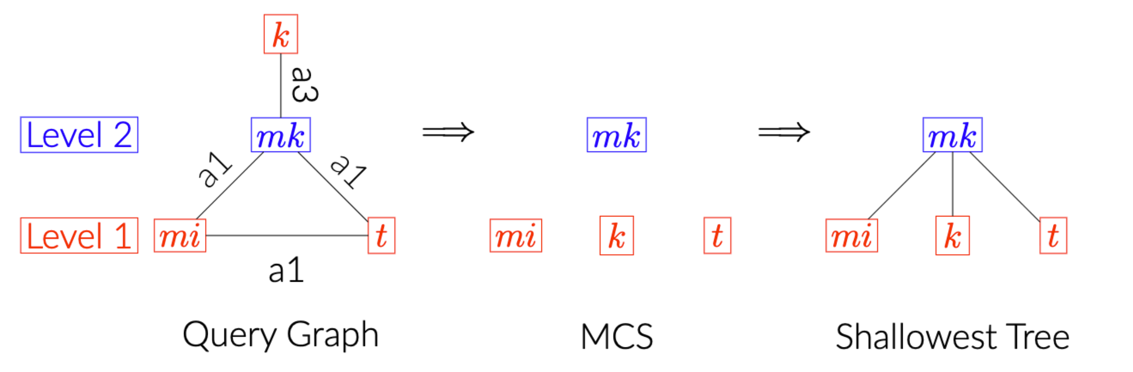
Now we are trying to understand how much this shallow and wide tree benefits the (approximate) semi-joins / predicate transfer, the parallelism and reduces the network cost of shipping filters/tables around, if any.