Linear-Time Selective Reduction

A query may contain many more relations and variables than both what we want to see in the final result and what we need for join and aggregation. Selective reduction is a process to trim away the irrelevant while evaluating a query. Tarjan and Yannakakis came up with a linear-time solution for acyclic queries. More specifically, their algorithm selectively reduce an acyclic query of $n$ variables and $m$ relations in $O(n + m)$ time.

Query as Hypergraph

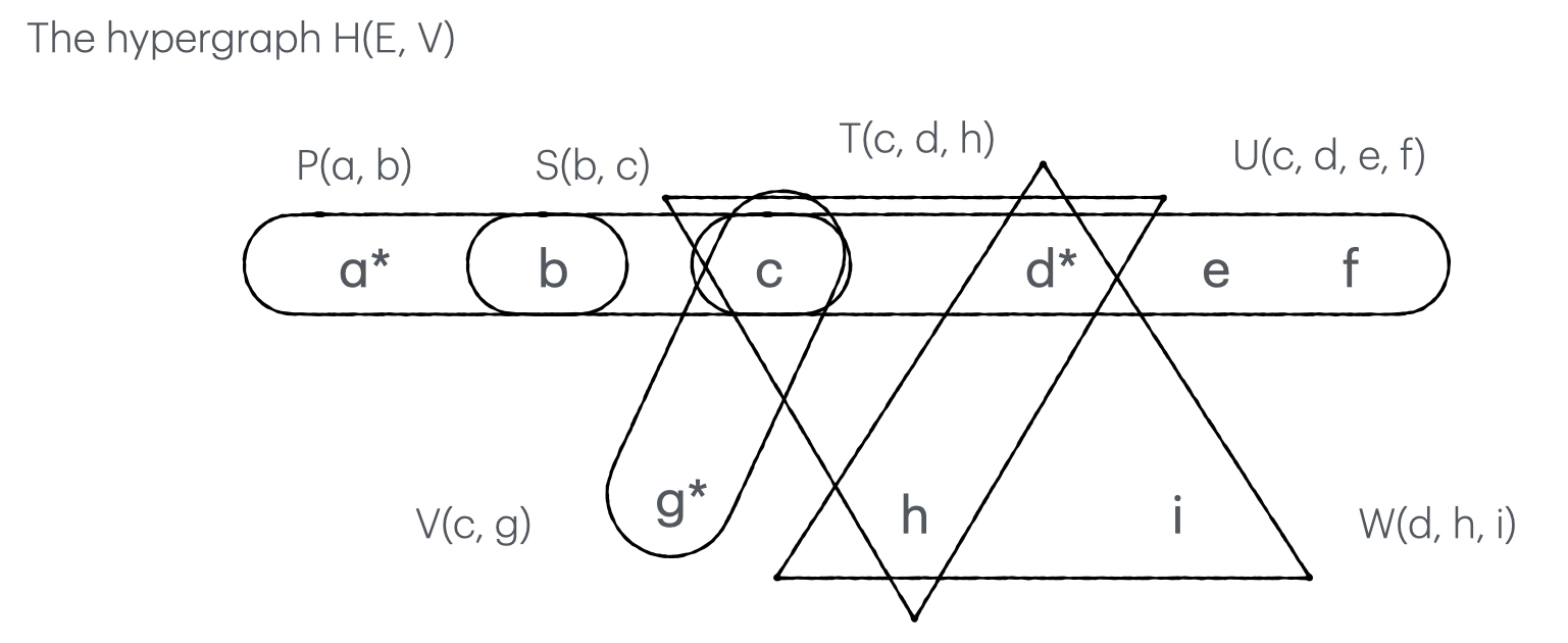
Let’s consider an acyclic query $Q(a, d, g) = P(a, b), S(b, c), T(c, d, h), U(c, d, e, f), V(c, g), W(d, h, i)$ where $a, d, g$ are free variables we’d like to see in the query result. All others are bound variables. We can derive the hypergraph below by regarding each variable as a vertex and each relation as a hyperedge.

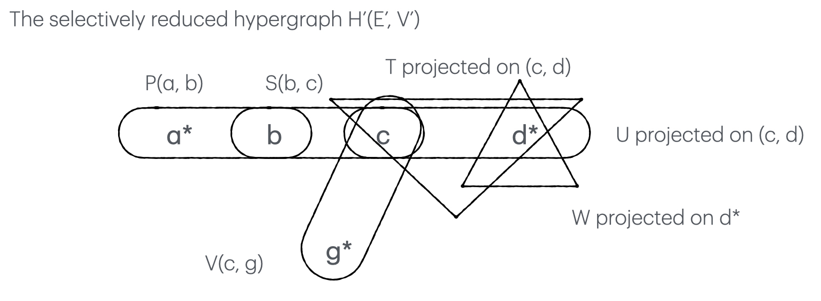
Selective reduction gives $Q(a, d, g) = P(a, b), S(b, c), V(c, g), \Pi_{c,d}T, \Pi_{c, d}U, \Pi_{d}W$ whose hypergraph is shown below.

The linear-time selective reduction consists of 2 steps. First, Max Cardinality Search, then, Repetitive Reduction.

Max Cardinality Search

To prepare for the reduction, Tarjan and Yannakakis found it neccesary to first number everything and proposed an algorithm, Max Cardinality Search (MCS). The algo numbers the vertices in a decending order, and simultaneously number the hyperedges in an ascending order.

Given a hypergraph, MCS follows a 4-step procedure:

1. Select the edge with the top priority (starting from an edge containing free variable & breaking ties by cardinality)
2. Number all vertices in the selected edge
3. Calculate the edge measurements
4. Update the priorities of its neighboring edges

The animated figure below shows the very beginning of an MCS. (1) It starts with the edge $P(a, b)$ which is numbered the 1st edge, $R(1)$. $a$ is assigned with 9, the number of vertices. At any point of the process, $i$ of $R(i)$ can be interpreted as the ‘timestamp’ of when an edge is selected. The smaller, the earlier.

MCS proceeds to (2) number all vertices in the selected hyperedge. Here, $b$ is numbered 8. For we only need the edge numbers for reduction, the order of numbering vertices in an edge does not really matter. Any permuation works.

The numbering of $R(1)$ is done when all of its vertices have been checked.

We take a quick pause after numbering each edge to calculate two key measurements useful in the later reduction process. Those of $R(1)$ are,

• $ \vert R(1) \vert = 2$ meaning that there are 2 vertices in $R(1)$;
• $ \vert R(1) \vert = 0$ meaning that none of them has been numbered before $R(1)$ is selected.

While numbering $R(1)$, we number the vertex $b$ that also appears in another edge $S(b, c)$. (4) We increment the priority of $S(b, c)$ by 1. Notice that the numbering of each vertex might increase the priorities of multiple edges.

We proceed to number the edge with the highest priority, $R(2)$.

In case that two or more edges have the highest priority, we break ties by cardinality (largest edge preferred). As we can see in the animated figure below, the numbering of $c$ increases the priorities of multiple edges, namely $T(c, d, h)$, $V(c, g)$ and $U(c, d, e, f)$, all to 1. The largest, $U(c, d, e, f)$, is selected as $R(3)$.

We repeat the above process until all vertices and edges are numbered as shown below.

As each vertex is numbered exactly once, and so is each edge, the time complexity of MCS is $O(n + m)$. The cardinality-based tie breaker may add a factor $log(m)$ to it.

Repetitive Reduction

Given a fully numbered hypergraph by MCS, we carry out the selective reduction by repeating the following 3-step procedure:

1. Delete any bound variable that belongs to exactly one edge
2. Update $ \vert R(i) \vert $ accordingly
3. Delete any $R(i)$ s.t. $ \vert R(i) \vert = \vert R’(i) \vert \text{ or } \vert R(i) \vert = \vert R’(i+1) \vert $

In the 1st round shown below, we can immediately (1) delete $e, f \in R(3)$ and $i \in R(5)$, each appearing in exactly one edge. Then we shall (2) update the corresponding $ \vert R(3) \vert $ and $ \vert R(5) \vert $ to 2, to reflect their up-to-date cardinality after deletion. (3) While looking for $ \vert R(i) \vert = \vert R’(i) \vert \text{ or } \vert R(i) \vert = \vert R’(i+1) \vert $, we find two candidates,

• $ \vert R(3) \vert = \vert R’(4) \vert $
• $ \vert R(5) \vert = \vert R’(5) \vert $

Let’s delete them one by one following a descending order of timestamp, starting with $R(5)$. The deletion creates a void in the timestamp sequence, between $R(4)$ and $R(6)$, and may reduce $ \vert R’(6) \vert $. In this case, $ \vert R(5) \vert - \vert R’(5) \vert = 0$ says that every vertex in it has been numbered by its previous edges. So the deletion does not reduce $ \vert R’(6) \vert $. To fill the void, we decrement the timestamp of $R(6)$ by 1, making it the new $R(5)$. We repeat the same drill for $R(3)$. $ \vert R(3) \vert - \vert R’(3) \vert = 1$ says that 1 vertex is numbered at timestamp 3. Due to the deletion, we shall associate $R(4)$ with every vertex numbered at both timestamp 3 and 4. To fill this void, we decrement $R(4)$ to $R(3)$ and $R(5)$ to $R(4)$. The 1st round is over.

We repeat the 3-step process in the 2nd round shown below. We can only (1) delete $h \in R(3)$ and (2) update $R(3)$, as no edge satisfies the condition $ \vert R(i) \vert = \vert R’(i) \vert \text{ or } \vert R(i) \vert = \vert R’(i+1) \vert $. The 2nd round is over.

As we can’t proceed any further, we wrap up the reduction.

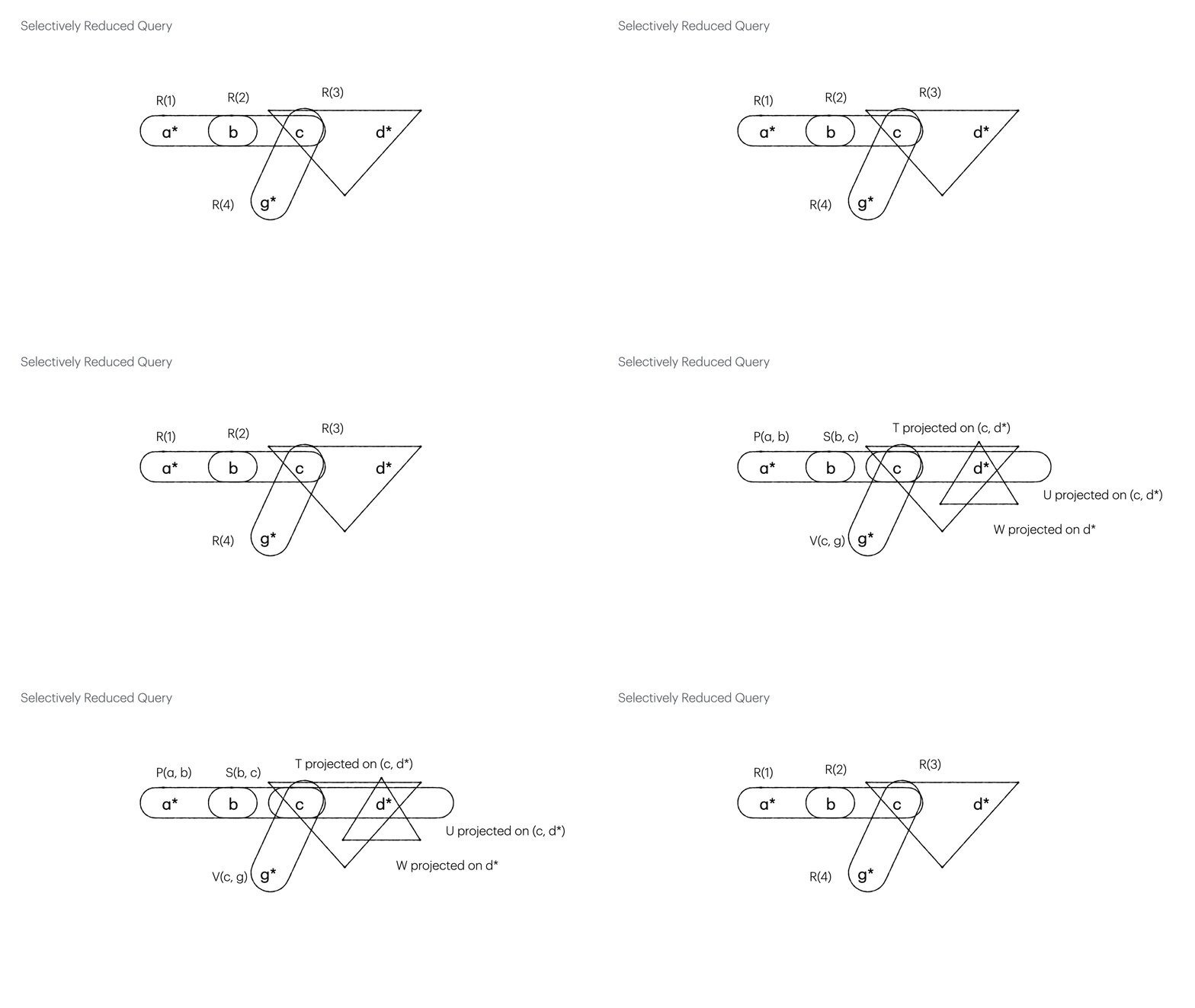
By putting back all the relations (edges) which can be projected onto the existing variables (vertices), we have the selectively reduced query.

The numbered edges expedite the check of the edges subsumed by others, bringing down the time complexity from $O(m^2)$ to $O(m)$.

To identify the vertices belonging to exactly one edge, it requires at least the maintenance of a min-heap that keeps the vertex appearing in the fewest edges, therefore adding another factor of $log(n)$.